In the previous article, we provided an introduction to dynamic pricing, explaining what it is, with examples, and discussing its benefits and implementation methods. In this article, we aim to delve into the more technical aspects in as clear terms as possible.
Although the term "optimization problem" may sound complex, it essentially means "calculating the best." In the context of dynamic pricing, it involves calculating the price that maximizes a store's revenue. However, dynamic pricing is not a one-size-fits-all technique; there are various types depending on the definition of "best." While many associate dynamic pricing with price calculations, it goes beyond that, allowing for solving advanced problems such as adjusting inventory levels based on production lead times. In this article, we'll introduce several examples of different types of dynamic pricing.
This is the simplest form of dynamic pricing. When you search for "dynamic pricing," most of the information you find likely explains this concept. Generally, the sales of a product are influenced by its price. Lower prices lead to higher sales, while higher prices result in fewer sales. The relationship between price and sales quantity (demand) forms a curve known as the demand curve (Figure 1).
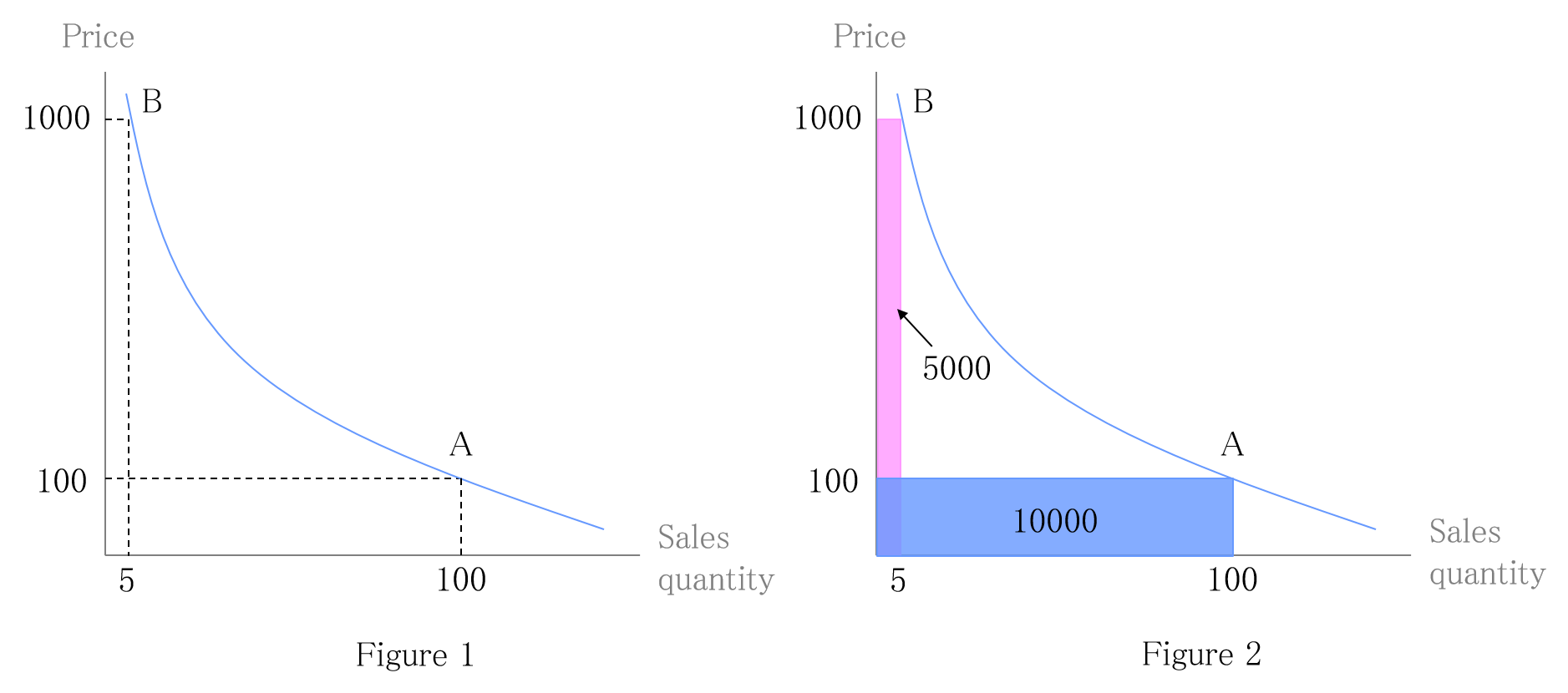
At point A in the graph, the price is set low (¥100), resulting in a high quantity sold (100 units). On the other hand, point B has a high price (¥1000), and only 5 units are sold. Now, which price is better?
Let's consider revenue maximization (Figure 2). The revenue at point A is ¥100 * 100 units = ¥10,000, whereas the revenue at point B is ¥1000 * 5 units = ¥5000. Therefore, point A yields higher revenue, making the ¥100 price more favorable than the ¥1000 price.
The rectangles at each point in the graph represent the revenue. Therefore, single-point revenue optimization seeks to find the point that maximizes the area of these rectangles, ultimately calculating the price that maximizes revenue.
In the previous article, we mentioned that dynamic pricing is suitable for "products whose value changes over time." In such cases, single-point revenue optimization faces challenges. For example, the value of an airline ticket becomes zero after the flight time. Even if the optimal price before the flight is ¥10,000, it cannot be maintained throughout. If all tickets are not sold before the flight, the remaining tickets will become wasteful. Therefore, if there are excess tickets just before the flight, it is more profitable to lower the price to ensure they are all sold.
In this case, the challenge is to adjust the price while considering the sales deadline and inventory level to avoid unsold products. More precisely, it becomes a problem of "maximizing the total revenue from the current point to the sales deadline." To solve this problem, you need to calculate the price that sells all remaining inventory within the remaining time until the sales deadline. Dyna-pricing employs mathematics to compute the optimal solution to this problem.
Both single-point revenue optimization and period total revenue optimization calculate optimal prices based on the demand curve. In other words, price calculation is not possible without information from past sales and demand data. However, for newly opened e-commerce stores, data for drawing a demand curve is not accumulated, and dynamic pricing cannot be utilized. This is known as the "cold start" problem.
Moreover, the demand curve is not always constant. The demand curve for sweaters changes with the seasons. Additionally, for the same product, the demand curve for a laptop will differ between business professionals and high school girls. It is impossible to prepare demand curves for all cases in advance, so there is a need for a mechanism to estimate them automatically.
Machine learning excels at extracting information from data. Dyna-pricing incorporates machine learning capabilities, learning from daily sales data even for newly opened stores and improving the accuracy of dynamic pricing. If customer attribute data is available, it is also possible to learn demand curves for each segment.
Furthermore, Dyna-pricing calculates the reliability information of the estimated price, addressing the cold start problem. When there is still limited data and the learning is incomplete, the presented price has low reliability. This allows for manual price adjustment or narrowing the price range according to reliability. Displaying price reliability information to customers enables them to anticipate price fluctuations, easing psychological burdens.
Introducing dynamic pricing can alter customer purchasing behavior and create challenges. For instance, in the case of an airline with many empty seats, customers may anticipate a reduction in ticket prices just before the flight, leading them to postpone purchasing until the last minute. In such cases, if sales do not progress until just before the flight, and inventory does not decrease, it triggers further price reductions. Since there is no sales data when data accumulation is insufficient, it also adversely affects machine learning.
This issue of delayed purchasing can be resolved by distinguishing between apparent demand and latent demand. Apparent demand refers to the demand actually reflected in sales data. On the other hand, latent demand refers to the demand that exists, but has not resulted in sales. The problem of delayed purchasing is included in this latent demand. If it is possible to know latent demand, the issue of delayed purchasing can be resolved.
Dyna-pricing learns latent demand by accumulating browsing data when customers view product pages in an e-commerce store. This enables robust pricing that is not affected by delayed purchasing.
While slightly different from the dynamic pricing explained so far, auctions are also a pricing method based on determining the price. Dynamic pricing calculates prices based on past sales and demand data, but for a unique item like a rare painting, there is no sales data to rely on, and dynamic pricing cannot be used.
Auctions, in the sense of determining the price, are a form of pricing technique. Auctions can determine the price even when past demand data is unknown by asking customers to bid on the "price they are willing to pay." However, the problem with auctions is that customers may not honestly disclose their willingness to pay. This is known as the problem of truthful reporting.
Various techniques have been studied in the field of auction theory to achieve truthful reporting. The most famous example that is actively used is Google's advertising auction. Matema has researchers well-versed in auction theory, and it is possible to design auctions tailored to specific business/products.
In this article, we explained some challenges of dynamic pricing and the technologies to address them. While there may not be much need to be aware of dynamic pricing in your daily life, it is advisable to consult with experts when customizing it for your products/business. We also accept consultations, so please feel free to contact us.